Review Notes for the Deep Learning Course

Review class video recording Notes from GRC and his friends

0. Question Types

Question Type	Quantity	Score
Short Answer	4	60
Design	2	25
Unknown Type	1	15

The teacher was secretive about the final question, “As long as you listened in class, you can still get some points.”

1. Outline

Chapter 2

• Master the stochastic gradient descent algorithm
• Master the batch gradient descent algorithm
• Understand regularization (L1, L2)
• Master the concept of Dropout, processing flow, etc.
• Master common theorems: NFL, Ugly Duckling, Occam’s Razor, etc.

Chapter 3

• Master Logistic regression, Softmax regression
• Master various common loss function formulas and their application scenarios, such as squared loss, cross-entropy loss, etc.
• Understand empirical risk and structural risk

Chapter 4

• Master the advantages and disadvantages of several common activation functions (Sigmoid, ReLU)
• Understand the basics of feedforward neural networks

Chapter 5

• Master the characteristics of convolutional neural networks (compared to fully connected networks)
• Convolutional networks: convolution kernel, feature map, number of color channels
• The role of pooling layers
• Parameter calculation of common typical CNN convolution structures (e.g., number of parameters in convolution layers, number of connections, output map size, etc.)
• Master residual networks (working principles, formulas, etc.)

Chapter 6

• Expression of RNN formulas
• Gradient vanishing and exploding problems in RNNs
  • Corresponding solutions
• Master sequence-to-sequence models (synchronous and asynchronous)
  • Specific applications (synchronous and asynchronous - Sentiment Analysis)
  • Formula expression
  • Advantages and disadvantages
• Master LSTM
  • The role and significance of the three gates
  • Advantages and disadvantages of LSTM compared to RNN
  • ‘Input and output
  • ‘LSTM can solve the gradient vanishing problem, similar to the processing method of residual networks
• Master GRU
  • Improvements compared to LSTM
  • ‘GRU formulas

Chapter 7 Network Optimization

• Improvement of learning rates
• Learning rate decay - just take a look
• Periodic adjustment - no need to look at formulas
• Key mastery: Adaptive adjustment: Adagrad, Adadelta, RMSProp
  • Master the formulas and principles of the three methods, focusing on the formulas
• Gradient optimization
  • Momentum method
  • Nesterov accelerated gradient
  • Adam algorithm
• Gradient clipping
• Network optimization in high and low dimensions

  Escape saddle points

• Three methods of data normalization
  • ‘Extract the correlation of related dimensions - whitening
• Master batch normalization and layer normalization (definition, method, specific operation method)
• Dropout

Chapter 8

• Master the attention model
  • Significance - why the attention model is needed
  • Formula
  • Processing flow, etc.
• Master the self-attention model
  • Significance - key mastery, improvement over previous teaching, KQV calculation, etc.
  • Formula
  • Processing flow
• Master Transformer (structure, technology, etc.)

Chapter 14

• Five elements of reinforcement learning
  • Fifth element: $\pi_s$ policy
• Two value functions: state value function, state-action value function
• Master policy iteration algorithm, value iteration algorithm, SARSA algorithm, and Q-Learning algorithm

Monte Carlo sampling

2. Overview of Machine Learning

Three Elements of Machine Learning

Model

Linear model Generalized linear model $$f(x;\theta) = w^{T}\phi (x)+b$$

Learning Criterion

In the linear regression model, all the following loss functions $\mathbb L$ are squared loss functions.

Expected risk is for real-world situations

However, the true data distribution cannot be obtained and can only be approximated by empirical risk:

When using empirical risk to approximate expected risk, generalization error occurs. Reducing generalization error requires two methods: optimization and regularization (damaging optimization, preventing overfitting). Structural risk adds a regularization term to empirical risk, and minimizing structural risk can solve (alleviate) the overfitting problem.

Optimization Methods

(Batch) Gradient Descent, Stochastic Gradient Descent, Mini-batch Gradient Descent, Early Stopping

(Batch) Gradient Descent

Batch gradient descent requires calculating the gradient of the loss function on each sample and summing them up during each iteration (the objective function is the risk function on the entire training set). When the number of samples 𝑁 in the training set is large, the space complexity is relatively high, and the computational cost of each iteration is also large.

Stochastic Gradient Descent

Batch gradient descent is equivalent to collecting 𝑁 samples from the true data distribution and using the gradient of the empirical risk calculated from them to approximate the gradient of the expected risk. To reduce the computational complexity of each iteration, we can collect only one sample at each iteration, calculate the gradient of the loss function for that sample, and update the parameters, which is stochastic gradient descent.

The difference between batch gradient descent and stochastic gradient descent is whether the optimization objective of each iteration is the average loss function of all samples or the loss function of a single sample. Due to its simplicity and fast convergence speed, stochastic gradient descent is widely used. Stochastic gradient descent introduces random noise into the gradient of batch gradient descent. In non-convex optimization problems, stochastic gradient descent is more likely to escape local optima.

Mini-batch Gradient Descent*

Regularization Methods

Regularization is a class of methods that improve generalization ability by restricting model complexity, thereby avoiding overfitting, such as introducing constraints, adding priors, early stopping, etc. Regularization methods include:

1. L-norm Regularization
2. Weight Decay
3. Early Stopping
4. Dropout
5. Data Augmentation
6. Label Smoothing

L-norm Regularization

Essentially, it introduces a constraint as a penalty. Thus, during optimization, one must consider the penalty (regularization term) in addition to the objective function.

L1 regularization applies the same penalty regardless of the size of the weights, causing smaller weights to become 0. The greatest effect of L1 regularization is to make a large number of parameters zero, sparsifying the model. L2 regularization heavily penalizes large weights and lightly penalizes small weights. The square of the L2 norm is generally introduced into the equation for convenience of calculation (as shown above).

Dropout

See Network Optimization - Dropout section for details $$mask(x) = \begin{cases} mx, \quad \text{training phase} \ px, \quad \text{testing phase} \ \end{cases}$$

Common Theorems

No Free Lunch Theorem (NFL): For iterative optimization algorithms, there is no algorithm that is effective for all problems (within a finite search space). If an algorithm is effective for some problems, then it must be worse than a purely random search algorithm for other problems. In other words, the effectiveness of an algorithm cannot be discussed without considering specific problems, and every algorithm has limitations. “Specific problems require specific analysis.”

Occam’s Razor Principle: “Entities should not be multiplied beyond necessity.” The idea of Occam’s Razor is very similar to the idea of regularization in machine learning: simpler models have better generalization ability. If there are two models with similar performance, we should choose the simpler one. Therefore, in the learning criteria of machine learning, we often introduce parameter regularization to limit model capacity and avoid overfitting.

Ugly Duckling Theorem: “The difference between an ugly duckling and a white swan is as great as the difference between two white swans.” This is because there is no objective standard of similarity in the world; all standards of similarity are subjective. From the perspective of size or appearance, the difference between an ugly duckling and a white swan is greater than the difference between two white swans; however, from the perspective of genes, the difference between the ugly duckling and its parents is smaller than the difference between its parents and other white swans. Here, the ugly duckling refers to a young white swan.

3. Linear Models

Reference: Comparison of Two Linear Models

Logistic Regression

In the book “Watermelon Book,” it is called logit regression, a commonly used model for binary classification problems.

This is an ordinary linear model: $f(x;w)=w^{T}x$ An activation function is introduced for nonlinear transformation, mapping the output to $[0,1]$ as the probability of predicting a positive example: $$p(y=1|x) = g(f(x;w))=\frac{1}{1+exp(-w^Tx)}$$ In fact, the value of $f(x;w)$ is the logarithm of the ratio of the posterior probabilities of sample x being a positive or negative example, called the logit: $$w^{T}x = \log \frac{p(y=1|x)}{p(y=0|x)}$$ The loss function uses cross-entropy: $$R(w) = -\frac{1}{N} \sum\limits_{i=1}^{N}(y_{i}\log (\hat y_{i})+(1-y_{i})\log (1-\hat y_{i})) $$ where $y_i$ is the true value (label), and $\hat y_{i}$ is the predicted value. The result of differentiation is the product of the input and the first-order loss, so the gradient descent update is as follows: $$w_{t+1} = w_{t}+ \alpha \frac{1}{N} \sum\limits_{i=1}^{N}x_{i}(y_{i}-\hat y_{i})$$

Softmax Regression

Multiclass Logistic Regression, a more general form of Logistic Regression

Add regularization to the risk function to constrain its parameters. Without adding a regularization term to limit the size of the weight vector, it may cause the weight vector to be too large, resulting in overflow.

Analyze why the squared loss function is not suitable for classification problems. In classification problems, labels do not have a continuous concept. The distance between each label is also meaningless, so the squared difference between the predicted value and the label cannot reflect the degree of optimization of the classification problem.

For example, in classification 1, 2, 3, the true classification is 1, and being classified into 2 and 3 should have the same degree of error, but the squared loss function’s loss is not the same.

① Inconsistent objective function: The goal of classification problems is to correctly classify samples into different categories, not to predict a continuous value. The goal of the squared loss function is to minimize the squared difference between the predicted value and the true value, which is inconsistent with the goal of classification problems. ② Sensitivity to outliers: The squared loss function is very sensitive to outliers. In classification problems, outliers usually indicate incorrect classification of samples, which means that incorrect classification of outliers will result in very high loss. Outliers are more common in classification problems because classification problems involve predicting discrete category labels, and outliers may cause larger errors. ③ Gradient vanishing: The squared loss function is prone to gradient vanishing problems in classification problems. Since the output of classification problems is a probability or category label, when using the squared loss function, the gradient may become very small, making it difficult for the model to learn or converge. ④ Non-differentiability: In classification problems, commonly used activation functions (such as sigmoid, softmax) are usually incompatible with the squared loss function. This is because the output produced by these activation functions is not continuous, while the squared loss function is differentiable for continuous outputs. Therefore, using the squared loss function in classification problems may lead to non-differentiable situations, making it impossible to use conventional optimization algorithms for training.

4. Neural Networks

Activation Functions

A qualified activation function should have the following properties:

• Continuously differentiable
• Simple and easy to compute
• The range is in a suitable interval

Sigmoid Series

Both are sigmoid-type functions with saturation:

• High computational cost
• Smooth output, no jumping values
• Differentiable everywhere
• Suitable for probabilities
• Gradient vanishing
• Centered at 0/not centered at 0

ReLU Series

Advantages - Low computational cost, only simple addition and multiplication - Biological plausibility: unilateral inhibition - Left saturation, derivative is 1 when x>0, alleviating gradient vanishing - Accelerates convergence speed of gradient descent Disadvantages Non-zero centering, causing bias in subsequent layers Dead ReLU problem: once improperly updated, it can never be activated (ELU can solve this)

Feedforward Neural Networks

The input layer is not counted in the number of network layers; the number of network layers refers to the number of hidden layers.

Universal Approximation Theorem

According to the universal approximation theorem, a feedforward neural network composed of a linear output layer and at least one hidden layer using an activation function with the “squeeze” property can approximate any function defined on a bounded closed set in real space with arbitrary precision, as long as the number of neurons in the hidden layer is sufficient. Neural networks can be used as a “universal” function, capable of performing complex feature transformations or approximating a complex conditional distribution.

5. CNN

Fully connected networks (FCN) have the following problems when processing images:

• Too many parameters
• Lack of local invariance Natural images have local invariance features, such as scale scaling, translation, rotation, etc., which do not affect their semantic information. Fully connected feedforward networks find it difficult to extract these local invariance features.

CNN Characteristics

CNNs are naturally suited for processing images:

1. Local Connection: Local connections significantly reduce the network’s parameters. When dealing with high-dimensional inputs like images, it is impractical for each neuron to be fully connected to all neurons in the previous layer. Instead, each neuron is only connected to a local region of the input data, and this connection’s spatial size is called the neuron’s receptive field, which is a hyperparameter, essentially the filter’s spatial size.
2. Weight Sharing: Parameter sharing in convolutional layers is used to control the number of parameters. Each filter is locally connected to the previous layer, and all local connections of each filter use the same parameters, which also significantly reduces the network’s parameters.
3. Spatial or Temporal Subsampling: Its role is to gradually reduce the spatial dimensions of the data, thereby reducing the number of parameters in the network, making computational resources less demanding, and effectively controlling overfitting. These characteristics give convolutional neural networks a certain degree of translation, scaling, and rotation invariance. Compared to feedforward neural networks, convolutional neural networks have fewer parameters.

Convolutional Layer

Convolution kernel size: The convolution kernel defines the size range of the convolution, representing the size of the receptive field in the network. The most common 2D convolution kernel is 3*3. Generally, larger convolution kernels have larger receptive fields, see more image information, and obtain better global features. However, large convolution kernels lead to a significant increase in computation, reducing computational performance. (Extremely large ones are FCNs) Stride: The stride of the convolution kernel represents the extraction precision. The stride defines the length of each convolution when the convolution kernel performs convolution operations on the image. For a size 2 convolution kernel, if the step is 1, there will be overlapping areas between adjacent step receptive fields; if the step is 2, there will be no overlap between adjacent receptive fields, and no information will be missed; if the step is 3, there will be a gap of size 1 pixel between adjacent step receptive fields, which to some extent means that information from the original image is missed. Padding: When the convolution kernel does not match the image size, it causes the image after convolution to be inconsistent in size with the image before convolution. To avoid this situation, boundary padding is required for the original image.

Feature Map is an image (or other feature map) after convolution, representing extracted features. Each feature map can be considered as a type of extracted image feature. To improve the representation ability of the convolutional network, multiple different feature maps can be used in each layer to better represent the features of the image. In the input layer, the feature map is the image itself. If it is a grayscale image, there is one feature map, and the depth of the input layer 𝐷 = 1; if it is a color image, there are three feature maps for RGB color channels, and the depth of the input layer 𝐷 = 3. The convolutional layer inputs feature maps of size $M \times N \times D$, outputs $M’ \times N’ \times D’$, and each output feature map requires 𝐷 convolution kernels and one bias. Assuming each convolution kernel is of size 𝑈 × 𝑉, a total of 𝑃 × 𝐷 × (𝑈 × 𝑉) + 𝑃 parameters are required. The size of the convolution output map: $$M’ = \frac{M-K+2P}{S}+1$$ Number of connections: Number of parameters × size of the output feature map plane $(M’ \times N’)$

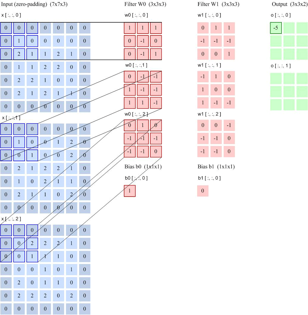
Taking LeNet-5 as an example for calculation:

Pooling Layer

Role:

1. Reduce computational load and number of parameters, making the model easier to train;
2. Lower the resolution of feature maps, reducing overfitting;
3. Extract more important features, as pooling layers only select maximum or average values, which often contain more information.

Residual Network

Question

Analyze the role of using a 1 × 1 convolution kernel in convolutional neural networks.

Answer

1. Dimensionality reduction (reduce parameters) In the Inception network Use 1 × 1 convolution to reduce the depth of feature maps
2. Dimensionality increase (use the least parameters to widen the dimension) As shown in the ResNet network structure diagram below The last layer on the right uses a 1 × 1 × 256 convolution kernel to increase the output from 64 dimensions to 256 dimensions And only requires 64_1_1*256 parameters
3. Cross-channel information interaction Achieving dimensionality increase and decrease operations is actually a linear combination between different channels, which is cross-channel information interaction
4. Increase non-linear characteristics After each convolution operation, a non-linear activation function is added. Using a 1 × 1 convolution kernel can increase non-linear characteristics without changing the scale of the feature map.

6. Attention Mechanism

Due to the limitations of optimization algorithms and computational capabilities, neural networks cannot be too complex to achieve universal approximation ability.

Attention

Significance

Solve the problem of long sequence semantic loss and input contribution distribution

1. Source passes through the Encoder, generating intermediate semantic encoding C.
2. C passes through the Decoder, outputting the translated sentence. In recurrent neural networks, y1 is generated based on C, then y2 is generated based on (C, y1), and so on. In traditional recurrent neural networks, y1, y2, and y3 are all calculated based on the same C. However, this may not be the best solution because different words in the Source have different influences (contributions) on y1, y2, and y3.

Starting from semantic encoding C, the attention mechanism allows it to adaptively change according to the encoder’s input at each moment, thereby affecting the output of the next module (e.g., decoder). AIM: Solve the problem of each input’s contribution.

Formula

Process

1. F(Q,K) calculates similarity, which can use Dot Product, Cosine, MLP
2. The output of F is normalized using Softmax to obtain attention distribution probabilities
3. Finally, calculate the weighted average of input information based on $a_i$ to obtain the attention value This diagram is no different from the previous one, just more concise and intuitive. Note that the weighted average after SoftMax can be written in the form of the expectation of a random variable.

Variants

Li Hongyi explained this key-value attention mechanism.

Multi-head attention mechanism.

Self-Attention

Significance

Introduce the Self-Attention mechanism, as the name suggests, referring to the Attention mechanism that occurs between elements within the Source or within the Target, which can also be understood as the Attention mechanism in the special case where Source = Target. The specific calculation process is the same as Soft Attention.

KQV Mode

Exactly the same as what Li Hongyi explained. The processing in SoftMax is slightly different, with the denominator being a constant.

Process

1. Calculate $k,q,v$ vectors, these three vectors are obtained by multiplying the input $X$ with the corresponding weight matrices $W^K,W^Q,W^V$
2. Calculate self-attention, obtained by dot product of Query and Key, this score determines the degree of attention to other parts of the input sentence when encoding a word at an unknown position
3. Divide the dot product result by a constant (usually $D_k=64$), then softmax the result to obtain the relevance of each word to the current word (maximum with itself)
4. Multiply the Value by the Softmax result and sum, the result is the self-attention value at the current node (scaled dot-product attention)

Transformer

Structure

The transformer adopts an encoder-decoder architecture, as shown in the figure below. The Encoder layer and Decoder layer are each composed of 6 identical encoders and decoders stacked together, making the model architecture more complex. Among them, the Encoder layer introduces the Multi-Head mechanism, allowing parallel computation, while the Decoder layer still requires serial computation.

Show-off

• Self-attention: Calculate the association of each word in the sentence with other words, helping the model better understand contextual semantics

• Multi-head attention: Each head focuses on different positions in the sentence, enhancing the expression ability of the Attention mechanism in focusing on the interactions between words within the sentence Why does the Transformer need Multi-head Attention? The original paper mentions that the reason for performing Multi-head Attention is to divide the model into multiple heads, forming multiple subspaces, allowing the model to focus on different aspects of information and finally integrate information from various aspects. Intuitively, multi-head attention helps the network capture richer features/information.

• Feed Forward Network (FFN): Introduces nonlinear transformation to the encoder, enhancing the model’s fitting ability

• The Decoder receives input from the output while also receiving input from the encoder, helping the current node obtain the content that needs to be focused on

• Feed Forward Network: After each layer goes through attention, there is also an FFN, whose role is spatial transformation. FFN consists of 2 linear transformation layers, with ReLu as the activation function in between. The addition of FFN introduces non-linearity (ReLu activation function), transforming the space of attention output, thereby increasing the model’s performance ability. The model can be used without FFN, but the effect is much worse. $$FFN(x) = ReLU(xW_{1}+b_{1})W_{2}+b_{2}=max(0,xW_{1}+b_{1})W_{2}+b_{2}$$

• Layer Normalization: Standardizes the optimization space, accelerating convergence $$LN(x_{i})=\alpha \frac{x_{i}-\mu_{i}}{\sqrt{\sigma^{2}+\xi}} + \beta$$

• Positional Encoding: Positional information encoding is located after the embedding of the encoder and decoder, before each block. It is very important; without this part, the model cannot run. Positional Encoding is a unique mechanism of the transformer, compensating for the inability of the Attention mechanism to capture the positional information of tokens in a sequence, allowing the positional information of each token to be fully integrated with its semantic information (embedding) and transmitted to all subsequent complex transformations of sequence representations.

• Mask Mechanism: Masking refers to covering certain values so that they do not affect parameter updates. The Transformer model involves two types of masks, namely padding mask and sequence mask. Among them, the padding mask is used in all scaled dot-product attention, while the sequence mask is only used in the self-attention of the decoder.

• Padding mask: The input sequence length may vary for each batch, requiring alignment of the input sequence.

  • Specifically, add 0 at the end of shorter sequences;
  • If the input sequence is too long, take the content on the left and discard the excess.
  • The attention mechanism should not focus on these, add a very large negative number (negative infinity) to these positions, so that after softmax, the probability of these positions will be close to 0.

• Sequence mask: Ensures that the decoder cannot see future information. For a sequence, at time_step t, the decoding output should only depend on the output before time t, not the output after time t. Therefore, information after t needs to be hidden. Generate an upper triangular matrix, where the upper triangle values are all 0. Apply this matrix to each sequence.

• Residual Network:

Network degradation phenomenon: When a neural network can converge, as the depth of the network increases, the network performance first gradually increases to saturation, then rapidly decreases.

In the transformer model, the encoder and decoder each have 6 layers. To ensure that the model can still achieve good training results when the number of layers is deep, a residual network is introduced into the model. Solves the network degradation problem caused by deep networks

Benefits

Seq2Seq model’s two pain points:

1. Long sequence, semantic disappearance problem
2. Positional information loss

• First, it improves the above two shortcomings, the approach is: 1-Residual structure, 2-Positional encoding
• Multi-head attention can extract more information
• The multi-head attention of the encoder layer can be calculated in parallel
• The self-attention module first “self-associates” the source sequence and target sequence, making the information contained in the embedding representation of the source sequence and target sequence itself richer
• The FFN layer also enhances the model’s expression ability
• …

7. RNN

SRN

Feedforward neural networks connect between layers, not within layers (not cyclic); both input and output are of fixed length and cannot handle variable-length sequence data.

$$h_{t}=f(Uh_{t-1}+Wx_{t}+b)$$ Turing completeness refers to a set of data operation rules that can achieve all the functions of a Turing machine and solve all computable problems. All Turing machines can be simulated by a fully connected recurrent network composed of neurons using the sigmoid activation function.

Bidirectional RNN is two RNNs stitched together, one reading a sentence (sequence) forward and one reading the sentence backward, so the output of each node contains information about the entire sentence.

Long-term Dependency Problem

Gradient explosion and gradient vanishing problems, can only learn short-period dependencies. Gradient explosion Weight decay: A regularization technique aimed at limiting model complexity. It is achieved by adding a regularization term to the model’s loss function, usually a penalty term for the L2 norm of the model weights. This penalty term acts to prevent the model weights from becoming too large, thereby reducing model complexity and suppressing model overfitting. Gradient clipping: Clip gradients greater than a threshold (e.g., >15 becomes 15) Gradient vanishing problem Change the cyclic edge to linear dependence: $h_{t} = h_{t-1}+g(X_{t};\theta )$ - This also solves the long-term dependency problem Add non-linearity (residual structure): $h_{t}= h_{t-1}+g(X_t,h_{t-1};\theta)$

The two structural improvements for the gradient vanishing problem are actually what LSTM does. LSTM can alleviate the gradient vanishing problem but cannot solve the gradient explosion problem (even worse because it is more complex). Regarding the LSTM gradient explosion problem, Li Hongyi explained that unlike the general situation where gradient vanishing is caused by the sigmoid function, the gradient vanishing in RNNs is because the same parameter is repeatedly used many times, like $x^n$, a small change in $x$ can cause a significant change in the result. The reason LSTM alleviates gradient vanishing is due to: cell memory, changing the cyclic edge from multiplication to addition, the influence of memory will always exist (unless the forget gate is activated), making memory more persistent.

LSTM

LSTM networks introduce a gating mechanism to control the information transmission path. The three “gates” are the input gate $i_t$, forget gate $f_t$, and output gate $o_t$, and their roles are:

• The forget gate controls how much information from the previous internal state $c_{t-1}$ needs to be forgotten (retained)
• The input gate controls how much information from the current candidate state $\tilde c_t$ needs to be saved (input)
• The output gate controls how much information from the current internal state $c_t$ needs to be output to the external state $h_{t}$

Advantages of LSTM compared to RNN:

The disadvantage is that the gradient still explodes!

Advantages of RNN:

• Has memory function, can process and predict time series data. Disadvantages of RNN:
• Performs poorly when processing long sequences because the gradient propagation is prone to gradient vanishing or explosion when the distance is long.
• Parameter update speed is slow because backpropagation needs to wait for the output result of the previous moment.
• Model capacity is small because the information propagation path is short, making it difficult to capture long-term dependency information. Advantages of LSTM:
• Can process long sequence information because LSTM stores long-term dependency information through memory cells, with a longer information propagation path.
• Parameter update speed is fast because long-term dependency information is stored in memory cells, allowing faster parameter updates.
• Model capacity is large because long-term dependency information is stored in memory cells, better capturing sequence information. Disadvantages of LSTM:
• Although LSTM can process long sequence information, performance is not as good as RNN when processing shorter sequences.

GRU

The spirit of Gate Recurrent Unit is: out with the old, in with the new. The input and output gates are linked, when the input is open, the output is closed, and vice versa, each time replacing with brand new data.

Seq2Seq ???

Specific Applications:

Formula Expression:

Synchronous:

Asynchronous:

8. Network Optimization

Challenges in Network Optimization

Structural differences No universal optimization algorithm Many hyperparameters Non-convex optimization problem Parameter initialization Escape local optima Gradient vanishing, gradient explosion

Non-convex optimization problems in low-dimensional space: There are some local optima (Local minima) and parameter initialization. Non-convex optimization problems in high-dimensional space (deep neural networks): The problem is not about escaping local optima, but about saddle points. Saddle points have a first-order gradient of 0, but the Hessian matrix is not semi-positive definite.

In high-dimensional space, the probability of a local minimum (Local Minima) being the lowest point in every dimension is very low, which means that most stationary points in high-dimensional space are saddle points. Stochastic gradient descent is very important for non-convex optimization problems in high-dimensional space. By introducing randomness in the gradient direction, it can effectively escape saddle points.

When a model converges to a flat local minimum, its robustness is better, meaning that small parameter changes will not drastically affect the model’s ability; whereas when a model converges to a sharp local minimum, its robustness is relatively poor. When training a network, it is not necessary to find the global minimum, as this may lead to overfitting.

Improvement methods for neural network optimization:

• Optimization algorithms
  • Dynamic learning rate adjustment
  • Gradient correction estimation
• Parameter initialization methods, preprocessing methods
• Modify network structure to optimize the landscape
• Hyperparameter optimization

Optimization Algorithms

Impact of Batch Size

Batch size does not affect the expectation of stochastic gradients, but it affects the variance of stochastic gradients; Large batch - small variance of stochastic gradients - stable - larger learning rate

Learning Rate Adjustment

Learning Rate Decay

Learning Rate Warm-up

In mini-batch gradient descent, when the batch size is set relatively large, a relatively large learning rate is usually required. However, at the beginning of training, since the parameters are randomly initialized, the gradients are often large, and combined with a relatively large initial learning rate, it can make training unstable. Therefore, a smaller learning rate is needed at the beginning stage, and then gradually restored (warmup). After warmup ends, the learning rate can be decayed again.

$$\alpha_{t}= \frac{t}{T}\alpha_{0}$$ where $T$ is the number of iterations for warm-up.

Periodic learning rate adjustment, including cyclic learning rate, warm restart, etc., involves first increasing and then decreasing within a cycle, with an overall decrease, which can handle sharp and flat minima, finding local optima.

Adaptive Learning Rate Adjustment

$\alpha$ is the learning rate, $\beta$ is the decay rate, and $\epsilon$ exists to prevent the denominator from being 0. Adagrad has a problem of monotonically decreasing learning rate. RMSProp changes the calculation method of $G_t$ from accumulation to exponential decay moving average, so the learning rate is no longer monotonically decreasing.

Gradient Optimization

Momentum

$$\Delta\theta_{t}=\rho\Delta\theta_{t-1}-\alpha g_{t}$$ where $\rho$ is the momentum factor, usually set to 0.9, $\alpha$ is the learning rate, and parameter update is $\theta_t = \theta_{t-1} +\Delta \theta_t$. The actual update difference of each parameter depends on the weighted average of the gradients over the recent period. When the gradient direction of a parameter is inconsistent over the recent period, the actual parameter update magnitude becomes smaller (end of training); conversely, when the gradient direction is consistent over the recent period, the actual parameter update magnitude becomes larger, playing an acceleration role (beginning of training).

Nesterov Accelerated Gradient

$$\theta = \hat \theta - \alpha g_{t}$$ $$\hat \theta = \theta_{t-1}+\rho \Delta \theta_{t-1}$$ To counter the version that Tang Chaogang easily misleads: $$\Delta \theta_{t} =\rho \Delta \theta_{t-1}-\alpha g_{t}(\theta_{t-1} +\rho \Delta \theta_{t-1}) $$ The real version:

The difference between the two is that Momentum uses the gradient at point $\theta_{t-1}$, while NAG uses the gradient at point $\hat \theta = \theta_{t-1}+\rho\Delta \theta_{t-1}$.

Nesterov completes in one step what Momentum does in two steps, hence the “acceleration.”

Adam

Adam ≈ RMSProp + Momentum

1. First calculate two moving averages $$M_{t}= \beta_{1}M_{t-1}+(1-\beta_{1})g_{t}$$ $$G_{t}=\beta_{2}G_{t-1}+(1-\beta_{2})g_t^2$$
2. Bias correction $$\hat M_{t} = \frac{M_{t}}{1-\beta_{1}^{t}}$$ $$\hat G_{t} = \frac{G_{t}}{1-\beta_{2}^{t}}$$
3. Update $$\Delta \theta = -\frac{\alpha}{\sqrt{\hat G_{t}+\epsilon}}{\hat M_t}$$

Gradient Clipping

Threshold clipping $$g_{t}= max(min(g_{t},b),a)$$ Clipping by norm $$g_{t} = b\frac{g_{t}}{\vert \vert g_{t} \vert \vert }$$

Parameter Initialization

• Pre-training
• Random Initialization
  • Gaussian Distribution (Normal)
  • Uniform Distribution
• Fixed Value Initialization

Data Preprocessing

Data Normalization

Max-min Normalization $$\hat x = \frac{x-min}{max-min}$$ Standardization $$\hat x = \frac{x-\mu}{\sigma}$$ Whitening and PCA After whitening, the correlation between features is low, and all features have the same variance. One main implementation method is PCA.

Batch Normalization and Layer Normalization

$$\hat x = \frac{x-\mu}{\sqrt{\sigma^{2}+\epsilon}}\gamma + \beta$$ The calculation is the same, but the objects are different:

Batch normalization is done between different samples, while layer normalization is done within the same sample. Batch normalization is the normalization of a single neuron for different training data, while layer normalization is the normalization of all neurons in a certain layer for a single training data.

Question

Exercise 7-8 Analyze why batch normalization cannot be directly applied to recurrent neural networks.

Answer

Layer normalization can be used for RNNs, as shown below to show the difference between the two

• Batch normalization is the normalization operation for a single neuron in an intermediate layer, so the number of mini-batch samples cannot be too small, otherwise it is difficult to calculate the statistical information of a single neuron (too few samples have no statistical significance).
• If the distribution of the net input of a neuron is dynamically changing in the neural network (such as RNN), then batch normalization cannot be applied.
• Layer normalization is the normalization of all neurons in an intermediate layer, and RNN can use layer normalization.

Question

Reference formula as follows

Answer

1. 𝑓(BN(𝑾𝒂(𝑙−1) + 𝒃)) indicates batch normalization after linear calculation and before non-linear activation (i.e., net input 𝒛(𝑙)).
2. 𝑓(𝑾BN(𝒂(𝑙−1)) + 𝒃) indicates batch normalization before linear calculation of the previous layer’s output, i.e., current layer.

Using the first batch normalization method can avoid changes in distribution due to linear calculation.

Dropout

Dropout: When training a deep neural network, we can randomly drop some neurons (and their corresponding connection edges) to avoid overfitting.

During training, the average number of activated neurons is 𝑝 times the original. During testing, all neurons can be activated, which causes inconsistency in network output during training and testing. To alleviate this problem, during testing, the input 𝒙 of the neural layer needs to be multiplied by 𝑝, which is equivalent to averaging different neural networks. The retention rate 𝑝 can be selected as the optimal value through the validation set. Generally speaking, for neurons in hidden layers, the retention rate 𝑝 = 0.5 works best, which is effective for most networks and tasks. When 𝑝 = 0.5, half of the neurons are dropped during training, leaving half of the neurons that can be activated, and the randomly generated network structure is the most diverse. For neurons in the input layer, the retention rate is usually set to a number closer to 1, so that the input changes are not too large. Dropping neurons in the input layer is equivalent to adding noise to the data, thereby improving the network’s robustness.

This PPT is still wrong, Qiu Xipeng’s book says there are $2^n$ sub-networks, and when he copied it, it became 2n 😅

The Bayesian explanation means that dropout is a sampling of the parameter $\theta$.

Variational dropout: When applying dropout to RNNs, dropout should not be applied to cyclic connections, but rather to non-cyclic connections randomly. Randomly drop each element of the parameter matrix and use the same dropout mask at all times.

Analyze why dropout cannot be directly applied to cyclic connections in recurrent neural networks? Randomly dropping each time step’s hidden state will damage the memory ability of the cyclic network in the time dimension.

9. Deep Reinforcement Learning

Five Elements

The basic elements of reinforcement learning include:

1. State 𝑠 is a description of the environment, which can be discrete or continuous, and its state space is 𝒮.
2. Action 𝑎 is a description of the agent’s behavior, which can be discrete or continuous, and its action space is 𝒜.
3. Policy 𝜋(𝑎|𝑠) is a function that determines the next action 𝑎 based on the environment state 𝑠. (Mapping from state to action)
4. State transition probability 𝑝(𝑠′|𝑠, 𝑎) is the probability that the environment transitions to state 𝑠′ at the next moment after the agent takes an action 𝑎 based on the current state 𝑠.
5. Immediate reward 𝑟(𝑠, 𝑎, 𝑠′) is a scalar function, i.e., after the agent takes an action 𝑎 based on the current state 𝑠, the environment will give the agent a reward, which is often related to the state 𝑠′ at the next moment.

Markov Process

A Markov process is a sequence of random variables $𝑠_0, 𝑠_1, ⋯, 𝑠_𝑡 ∈ 𝒮$ with the Markov property, where the next state $𝑠_{𝑡+1}$ depends only on the current state $𝑠_𝑡$, $$𝑝(𝑠_{𝑡+1}|𝑠_𝑡, ⋯ , 𝑠_0) = 𝑝(𝑠_{𝑡+1}|𝑠_{t}),$$ A Markov decision process adds an additional variable: action $𝑎$, where the next state $𝑠_{𝑡+1}$ depends not only on the current state $𝑠_𝑡$ but also on the action $𝑎_𝑡$, $$𝑝(𝑠_{𝑡+1}|𝑠_𝑡,a_t, ⋯ , 𝑠_0,a_0) = 𝑝(𝑠_{𝑡+1}|𝑠_{t},a_t),$$ where $𝑝(𝑠_{𝑡+1}|𝑠_{t},a_t)$ is the state transition probability.

There are no actions and rewards in a Markov process, while a Markov decision process considers actions and returns.

Given a policy $𝜋(𝑎|𝑠)$, a trajectory $\tau$ of a Markov decision process is $$\tau = 𝑠_0, 𝑎_0, 𝑠_1, 𝑟_1, 𝑎_1, ⋯ , 𝑠_{𝑇−1}, 𝑎_{𝑇−1}, 𝑠_{𝑇 }, 𝑟_𝑇$$ The probability of obtaining this trajectory is: $$p(\tau )= p(s_0)\prod_{t=0}^{T-1}\pi(a|s)p(s_{t+1}|s_{t},a_{t})$$ If the environment has no terminal state, the return of the entire trajectory is: $$G(\tau ) = \sum\limits_{t=0}^{T-1}\gamma^tr_{t+1}$$ where $\gamma \in [0,1]$ is the discount rate. When $\gamma$ is close to 0, the agent cares more about short-term returns; when $\gamma$ is close to 1, long-term returns become more important. When calculating, unless otherwise specified, take $\gamma =1$. The objective function of reinforcement learning is to maximize the expected return.

Value Function-based Learning Methods

State value function: The expected return obtained by executing policy $\pi$ starting from state $s$.

$$V^{\pi}(s) =\mathbb E{{\tau \sim p(\tau)} }{[\sum\limits{t=0}^{T-1}\gamma^{t}r_{t+1}\vert \tau_{s_{0}}= s]}$$

The expected return of a policy $\pi$ is (the expectation of all possible trajectories, the expectation of all state values that can be reached from s) $$\mathbb E{\tau}{[G(\tau)]} = \mathbb E{{s\sim p(s_0)}}[V^{\pi}(s)]$$ $s$ transitions to $s^\prime$, there is a Bellman equation, $$V^{\pi}(s) = \mathbb E{{a\sim\pi(a|s) }}\mathbb E{{s’\sim p(s’|s,a) }}[r(s,a,s^\prime)+\gamma V^{\pi}{(s^{\prime})}]=\sum\limits_{a\in A}\pi(a|s)(R_{s}^{a}+{\gamma}\sum\limits_{s’\in S}P_{ss’}^{a}V^{\pi}(s’))$$ Imagine a Markov chain to help remember this formula. Inside, $\pi(a|s)$ is the policy, which is the probability distribution of taking action $a$ in state $s$, and $p$ is the probability distribution of the state $s$ possibly reaching state $s’$.

Q function: More detailed, the expected total return obtained by taking action $a$ in state $s$ and then executing policy $\pi$: $$Q^{\pi}(s,a) = \mathbb E{{s’\sim p(s’|s,a) }}[r(s,a,s^\prime)+\gamma V^{\pi}{(s^{\prime})}]=\sum\limits{s’\in S}P_{ss’}^{a}(R_s^a+\gamma V^{\pi}{(s^{\prime})})$$ It is equivalent to fixing the action $a$ in the Bellman equation. The state value function $𝑉^𝜋(𝑠)$ is the expectation of the Q function $𝑄^𝜋(𝑠, 𝑎)$ with respect to action 𝑎, i.e., $V^{\pi}(s) = \mathbb E_{a\sim \pi (a,s)}{[Q^{\pi}(s,a)]}$, substituting into the above equation, we get the Bellman equation for the Q function: $$Q^{\pi}(s,a) = \mathbb E_{s’\sim p(s’|s,a)}{[r(s,a,s’)+\gamma \mathbb E_{a’ \sim \pi(s’,a’)}{[Q^{\pi}(s’,a’)]}]}$$

Dynamic Programming Methods

Both methods are model-based reinforcement learning (model-dependent reinforcement learning), where the model is a Markov decision process (MDP). Two limitations:

• Requires a known model, i.e., the state transition probability 𝑝(𝑠′|𝑠, 𝑎) and reward function 𝑟(𝑠, 𝑎, 𝑠′) of the Markov decision process must be given. However, this requirement is difficult to meet in practical applications (solution: random walk to explore the environment).
• Large state space, extremely low efficiency (solution: neural network approximate calculation of V (deep belief Q network)).

Policy Iteration

Policy iteration includes policy evaluation (calculate $V^{\pi}(s)$) and policy improvement (simple greedy) two parts.

Value Iteration

It is equivalent to only iterating $V^{\pi}(s)$, the policy is not iterated, and it is directly generated at the end.

Monte Carlo Methods

Monte Carlo (sampling) methods: State transition probability 𝑝(𝑠′|𝑠, 𝑎) and reward function 𝑟(𝑠, 𝑎, 𝑠′) are unknown, the MDP model collapses (model-free reinforcement learning), and Q function needs to be calculated through sampling. $$Q^{\pi}(s,a) = \frac{1}{N}\sum\limits_{n=1}^{N}G(\tau^{n}{s_0=s,a{0=a}})$$ The Q function is approximated by the average return of N experimental trajectories. $\epsilon$-greedy method: Choose other actions in $\mathbb A$ with a probability of $\epsilon$ (very small), and each action is chosen with a probability of $\frac{\epsilon}{\vert \mathbb A \vert}$.

Temporal Difference Method

It is a same-policy method. Monte Carlo methods require a complete path to know the total return and do not rely on the Markov property; while temporal difference learning methods only need one step, and the total return needs to be approximately estimated through the Markov property.

Q-Learning

It is an off-policy temporal difference method. Unlike the SARSA algorithm, the Q-learning algorithm does not select the next action $𝑎′$ through $\pi^\epsilon$, but directly selects the optimal Q function, so the updated Q function is about policy $\pi$, not policy $\pi^\epsilon$.

Actor-Critic

10. 20th Grade Exam

Short Answer Questions

1. CNN Calculation

Input image 97973, 15 filters of 9*9, no zero padding, stride of 2.

1. Calculate the size of the output image (5 points)
2. The number of parameters in the convolutional layer (5 points)
3. Characteristics of CNN (5 points)

2. Self-Attention Mechanism

······ChatCPT·····Elon Musk·······Dangerous AI······

1. Structural diagram of the self-attention model (5 points)
2. If using dot product to calculate similarity, give the complete calculation process of self-attention (10 points)

3. Explain Theorems

Explain the No Free Lunch Theorem and the Ugly Duckling Theorem separately (10 points)

4. Optimization Algorithms

Explain the momentum method and Nesterov accelerated gradient (10 points)

5. Optimization Algorithms

Explain the difficulties and focus of parameter optimization in high and low dimensions (10 points)

Short Answer Questions

1. Describe the SGD algorithm and write down its advantages and disadvantages (10 points)
2. LSTM is an improvement over RNN, can it solve the gradient vanishing and gradient explosion problems? Please explain the principle (15 points)

Essay Question

….Xpeng Motors G6 autonomous driving is very powerful…. Suppose you are an algorithm engineer at Xpeng, please use deep reinforcement learning to model Xpeng’s human-machine dialogue system, list the five elements of reinforcement learning, and provide an algorithm to maximize the reward function. (15 points)

That’s right, deep reinforcement learning dialogue system;